The easiest way to script an Abaqus model is to set up or change the input file (.inp) with a script. For that, we just have to change and then run the .inp with Abaqus. This works well if you want to change the material or the boundary conditions, but not for geometries that have to be remeshed.
For each load case, the input file has to be changed and run with the Abaqus solver. Changing the .inp can be done with any programming language. Here, we do it using Python.
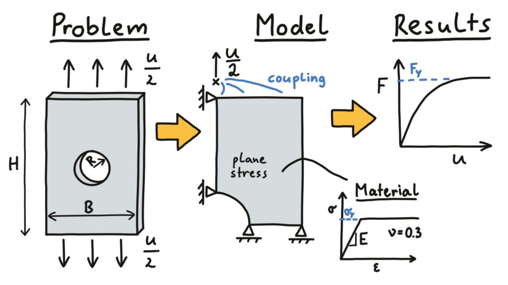
a) The example model
This is the model that we will use. It is a plate with a circular hole in the centre. In our input file, the geometry has already been meshed. We want to vary the yield stress σy between 500 MPa and 1500 MPa in 5 Steps and then evaluate plastic strains.
I prepared this inp-file of the model: pull_plate_original.inp
In this input file, node and element results are written into the dat file using the following lines:
** print node and element results into dat-file
*NODE PRINT
U, RF,
*EL PRINT
S, COORD, PEEQ,Code language: plaintext (plaintext)
As far as I know, you cannot find those commands in Abaqus CAE, but all the printing options to the dat file are given in section 4.1.2 of the Abaqus Documentation. The part of the material goes like this, where after the keyword *PLASTIC, lines of stress & plastic strain pairs are given. So our initial yield stress is 500 MPa and we have ideal plastic behaviour because, after the last line, ideal plastic behaviour is modelled:
*Material, name=steel
*Elastic
210000., 0.3
*Plastic
  500.,0.Code language: plaintext (plaintext)
Those are the results of the vertical stress and the plastic strain of the original input file:
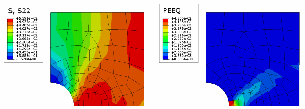
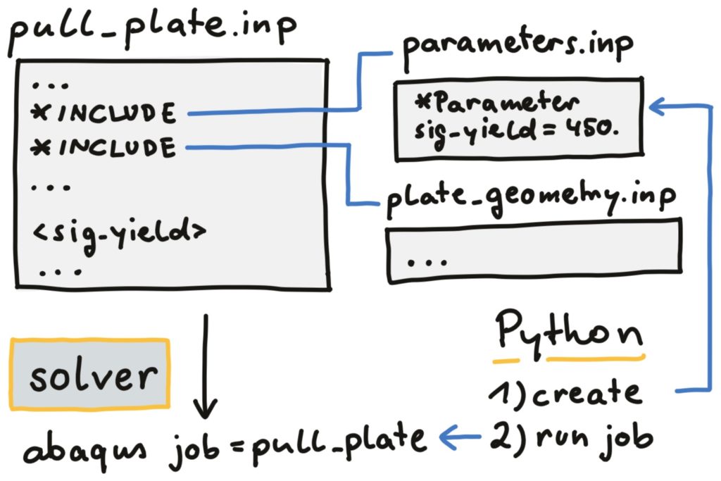
b) Preparing the input file
We prepare our input file in a way to better manipulate it later. This is just cosmetical, but working in a clean and structured way is most important in programming. First, we take the whole part and assembly definition and put it into a separate inp file called plate_geometry.inp. We will not change this inp file again and replace the lines that went into the plate_geometry.inp file by this *INCLUDE statement in the original inp file:
*INCLUDE, input=plate_geometry.inpCode language: plaintext (plaintext)Check now if the input file still runs. Also, we want to replace the yield stress in our input file. The most elegant way to do so is using the keyword *Parameter to define parameters in our input file (see Section 4.1.1 of the Abaqus Documentation for details) that we can use in the rest of the model with writing <parameter-name>.
*Parameter
sig_yield = 500.
**
*Material, name=steel
*Elastic
210000., 0.3
*Plastic
  <sig_yield>,0.Code language: plaintext (plaintext)
Also, we better put the parameter definition in another input file (parameters.inp) so we can change it easier. So we will not touch the main and the geometry input file later. This yields the remaining a prepared pull_plate.inp file like this:
*Heading
** plate with hole model, SI units
*Preprint, echo=NO, model=NO, history=NO, contact=NO
**
*INCLUDE, input=parameters.inp
*INCLUDE, input=plate_geometry.inp
**
*Material, name=steel
*Elastic
210000., 0.3
*Plastic
  <sig_yield>,0.
**
** Name: x_sym Type: Displacement/Rotation
*Boundary
plate-1.x_sym, 1, 1
** Name: y_sym Type: Displacement/Rotation
*Boundary
plate-1.y_sym, 2, 2
** -------------------------------------------------
*Step, name=pull_y, nlgeom=YES
*Static
1., 1., 1e-05, 1.
**
*Boundary
plate-1.RP, 1, 1
plate-1.RP, 2, 2, 0.08
plate-1.RP, 6, 6
**
*Output, field, variable=PRESELECT
*Output, history, variable=PRESELECT
** print node and element results into dat-file
*NODE PRINT
U, RF,
*EL PRINT
S, COORD, PEEQ,
*End StepCode language: plaintext (plaintext)
c) Manipulating the input file
We now need a script that writes parameters.inp files and then runs our main input file. To be able to later look in the odb files, we use job names like ‘plate-s_yield-500’. Let’s look at how to do that in Python. If you have Anaconda installed on your computer (which I highly recommend: it’s free and has the most important Python modules and tools), you can use interactive Jupyter notebooks or the development environment Spyder to develop a similar code for yourself.
I will not explain all the Python commands in detail; for that, you can look them up in the Python documentation. Note that I will only show the resulting Python code in the following. Actually, I build it up step by step and checked at every point if the latest part of the code did what I wanted it to. Which you should also do when you start with the exercises.
We assume that we already know all our input file parameters in the Python file and thus just create a new parameters.inp file from scratch. Since this file is replaced for each load case, we also write a separate file like this for each parameter set, ending with '_par.inp'. So we write in Python:
sig_yield = 500.
# use the yield stress in the job name
job_name = 'plate-s_yield-'+str(sig_yield)
# create the string for the parameters.inp file
# '\n' denotes a line break
par_string = '*Parameter\nsig_yield={}'.format(sig_yield)
# write to the parameters.inp file
with open('parameters.inp','w') as f:
    f.write(par_string)
# write to the ..._par.inp file
with open(job_name+'_par.inp','w') as f:
    f.write(par_string)Code language: Python (python)
So everything is ready for our job to run. With the command abaqus interactive input=pull_plate job=jobname we run this input file but use the jobname for our result files. In Python, running a command in the command line works best with subprocess.call('...', shell=True). As you can see, I also put everything into a neat function.
from subprocess import call
def make_inp_file(sig_yield):
    # use the yield stress in the job name
    job_name = 'plate-sig_yield-'+str(int(sig_yield))
    # create the string for the parameters.inp file
    # '\n' denotes a line break
    par_string = '*Parameter\nsig_yield={}'.format(sig_yield)
    # write to the parameters.inp file
    with open('parameters.inp','w') as f:
        f.write(par_string)

    # write to the ..._par.inp file
    with open(job_name+'_par.inp','w') as f:
    f.write(par_string)
    # run the inp file (subprocess.call)
    call('abaqus interactive input=pull_plate_original job='+job_name,
         shell=True)
    returnCode language: Python (python)
We can test the function calling it with a sinlge yield stress value of 380 MPa:
# call the function once
make_inp_file(sig_yield=380.)Code language: Python (python)
We can also create a list of interesting σy values and use a for loop to run the input file several times with those σy values:
# create list of sy values
sy_list = [500., 750., 1000., 1250., 1500.]
# run the inp-files for each sy value
for sy in sy_list:
    make_inp_file(sig_yield=sy)Code language: Python (python)
If you only have Abaqus and no separate Python installation on your computer, you can run this script (e.g. called run_inp_models.py) from the command window (the path to the Abaqus commands, usually something like C:\SIMULIA\Abaqus\Commands, needs to be in the environment variable path):
abaqus python change_inputs.pyCode language: Bash (bash)If you run it for the second time and the result files already exist, it will ask you for each run if you want to overwrite the existing job files. At this point, before running the Python file again, you should manually take the last job files and delete or move them to a different folder. Later, we will learn how to automatically delete the files before running Abaqus.
d) Reading data from dat-file
As I mentioned when looking at the inp file, we can write node and element results to the dat files. Reading them from those plain text files is nothing you would actually do after finishing this hole course, but let us look at that anyways.
Opening one of the dat files, we see that there are regions for the different increments of the model with some lines stating the increment information, for example, increment 17:
 INCREMENT    17 SUMMARY
 TIME INCREMENT COMPLETED  3.109E-03,  FRACTION OF STEP COMPLETED   1.00
 STEP TIME COMPLETED       0.100    ,  TOTAL TIME COMPLETED        0.100   Code language: plaintext (plaintext)
Then, the element output and the node output in this increment is listed for all nodes and elements. Let’s try to read the reaction force in the vertical direction (RF2) of the reference point in the last increment. And since this is something you would not regularly do, we take a quick-and-dirty approach.
The reference node has the number 91. In the dat file, you can see that the line giving the node output for node 91 looks like that (stating the node number, U1, U2, UR3, RF1, RF2, and RM3):
91 0.0000000E+00 1.0000000E+00 0.0000000E+00 ...Code language: plaintext (plaintext)So there are 9 spaces before the ’91’ so we can load the dat file, split it into lines and look for lines that start with ' 91 ':
with open('plate-s_yield-1500.dat','r') as f:
    lines = f.read().split('\n')
rp_lines = []
for line in lines:
    if line.startswith('         91 '):
        rp_lines += [line]
print(rp_lines)Code language: Python (python)
Now comes the quick-and-dirty part of reading the results. We split the last line at spaces to separate the values. But this also return lots of empty strings for spaces next to each other. So we delete those. Then we take the 6th string or the second to the last string in the list and convert that string to a float.
# result for last frame
res_line = rp_lines[-1]
# split ste string and delete empty strings from list
res_line = [i for i in res_line.split(' ') if i != '']
# take the second from last string (RF2) and convert it to a float
res_rf2 = float(res_line[-2])Code language: Python (python)
So we just read one result value from out dat file. If you got confused by all the string operations, do not worry! With Abaqus CAE we can evaluate results much easier!
e) Putting it all together
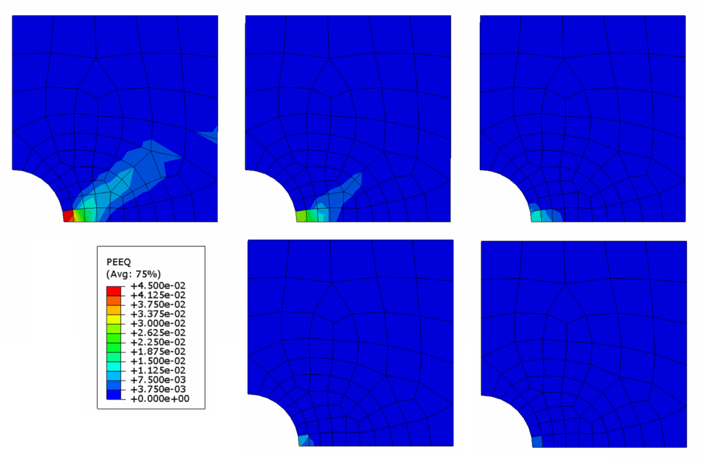
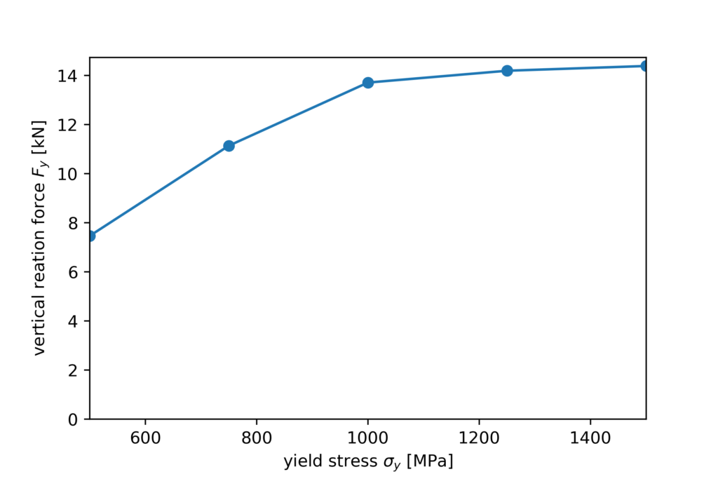
You can put that together into a function evaluate_rf2 that takes the name of the dat file as input and returns the rf2 value. See this function below. Adapting, running, and evaluating an inp file is then done in the function mak_inp_file that puts the results for the varied σy values into a dictionary that is printed at the end. When you run it, you see how the reaction force increases with increasing yield stress:
def evaluate_rf2(dat_file):
    # open the dat file with results in it
    with open(dat_file+'.dat','r') as f:
        lines = f.read().split('\n')
    # take the lines with reference point results
    rp_lines = []
    for line in lines:
        if line.startswith('         91 '):
            rp_lines += [line]
    # result for last frame
    res_line = rp_lines[-1]
    # split ste string and delete empty strings from list
    res_line = [i for i in res_line.split(' ') if i != '']
    # take the second from last string (RF2) and convert it to a float
    return float(res_line[-2])

def make_inp_file(sig_yield):
    # use the yield stress in the job name
    job_name = 'plate-s_yield-'+str(sig_yield)
    # create the string for the parameters.inp file
    # '\n' denotes a line break
    par_string = '*Parameter\nsig_yield={}'.format(sig_yield)
    # write to the parameters.inp file
    with open('parameters.inp','w') as f:
        f.write(par_string)
    # write to the ..._par.inp file
    with open(job_name+'_par.inp','w') as f:
        f.write(par_string)
    # run the inp file (subprocess.call)
    call('abaqus interactive input=pull_plate job='+job_name,
         shell=True)
    # read from the dat-file
    rf2 = evaluate_rf2(job_name)
    print('sig_yield = {} MPa: rf2 = {} N'.format(sig_yield,rf2))
    return rf2
# create list of sy values
sy_list = [500., 750., 1000., 1250., 1500.]
result_dict = {}
# run the inp-files for each sy value
for sy in sy_list:
    result_dict[sy] = make_inp_file(sy)
print(result_dict)Code language: Python (python)
We again run this code (including the function for evaluating the RF2 value) with the following line in the command window:
abaqus python run_input_models_eval.pyCode language: Bash (bash)We can plot the results obtained in this way and see that there is a rather nonlinear dependence of the vertical force on the yield stress:
Exercises
- Take the input file from the model you set up in chapter 2 and think about what value would be interesting to vary that is not related to the geometry. And what result value would be interesting to look at (preferably a node- or element result). Carry out all the above steps with your input file.
- Draw a curve using Python (as described in chapter 6) that relates your result value to your varied parameter. Would you have expected that?