As we looked into scripting the model in the last section, we now deal with the evaluation of the model in a scripted way. This can be done in the Abaqus Viewer, which is also included in Abaqus CAE. Everything starts now with the session repository. We can get the recorded commands from either the .rpy file or the abaqusMacros.py file.
There are two kinds of output in Abaqus:
- Field Output (result fields like displacement or stress)
- History Output (lists of result values like total strain energy for all time frames)
I) Stuff we want to evaluate
We would like to use the field output to export the data, view the result fields to write images, and look for maximum or mean result values in the model. We need the history output to export the data and create time-output curves.
Furthermore, in the Abaqus Viewer, you can create a path and evaluate field output along this path. The path points can be nodes selected by the user or coordinates that might or might not lie on the mesh. If you use a coordinate-based path, Abaqus has to interpolate the field output and returns nothing for points that lie outside the mesh.
There is some default output that is generated in each CAE model. If you need something that is not in the default output, you can define that in your model by creating an additional field output (like the integration point volume IVOL) or history output (like the displacement in the 1-direction U1 of the nodes in the set Set-1) in the step module of Abaqus CAE (with the model defined as m)
# additional field output
m.FieldOutputRequest(name='F-Output-2',
       createStepName='Step-1',variables=('IVOL',))

# additional history output: U1 for nodes in set
m.HistoryOutputRequest(name='H-Output-2',
	createStepName='Step-1', variables=('U1', ),
	region=inst.sets['Set-1'])Code language: Python (python)
To plot field output outside Abaqus, you need the coordinates of the nodes (node-based results like displacement) or the integration points (integration-point based results like stress). The easiest way to get those coordinates is defining coordinates as an additional field output (COORD). For the nodes, this can be done in Abaqus CAE and thus directly with Python; for the integration points, this has to be written to the inp file, which can be done in Abaqus CAE using the following commands (we also output the integration point volumes and node coordinates):
model.keywordBlock.synchVersions()
block_list = model.keywordBlock.sieBlocks
pos_i = [i for i, j in enumerate(block_list) if 'Output, field' in j]
# coordinates of IP (COORD) & volume of IP (IVOL)
str_out = "**\n*Element Output, directions=YES\n\
           COORD,IVOL,\n**\n*Node Output\nCOORD,"
# insert the str_out string
model.keywordBlock.insert(pos_i[0], str_out)Code language: Python (python)
Writing lines to the input file in Abaqus CAE is something you should do last before submitting the job because changing something in your model later usually messes up your model.
The first decision to make for the evaluation is whether to use Abaqus CAE or the Abaqus Viewer, which can be opened separately. I suggest to take Abaqus CAE as well, and if you build, run and evaluate your model in the same script, you need to do that anyway. With our usual import statements from the model, we have everything imported that we need for evaluation in Abaqus CAE.
Our first command is for loading the odb that we can view or get data from (you have the name of the odb in a variable called odb_name):
# open the odb with the odb_name
odb = session.openOdb(name=odb_name+'.odb')Code language: PHP (php)
Note that having many odb files open at the same time is not a good idea, so after you finished your evaluation, you should close the odb:
# close the odb
odb.close()Code language: PHP (php)
Usually, you would open an odb file and look at field outputs and maybe create some rather ugly-looking diagrams from history output. We now look into how to access field and history output with Python commands. Only some of it can be done by recording commands from Abaqus, so we need to take a closer look:
II) Obtaining field ouptut data
Let‘s access field output, which is a field of a result variable and thus exists for a big number of nodes or elements. The field output is part of its frame in the odb and and identified by a string (‘S’ for stress, ‘U’ for displacement, etc.): frame.fieldOutputs['S']. The results of the in the field output can then be accessed by the keyword values[i]: These values contain the node or element number, other information, and most importantly, our result data as a list. Note that the index i does not correspond to the element or node label. Here we take the last step and the last frame of it (an index of -1 returns the last element of a list) and get the stress for this last frame:
import numpy as np

# last frame
frame_end = odb.steps.values()[-1].frames[-1]
# obtain the field output for the stress 'S'
field_out = frame_end.fieldOutputs['S']

# getting field output directly (slow, but robust)
# and convert to numpy array
s_out = np.array([i.data for i in field_out.values])Code language: Python (python)
This way, we obtained a NumPy array of all stresses: Each line contains the 4 (2-d model) or 6 (3-d model) stress components.
There is also the possibility of using so-called BulkDataBlocks to access the result data. For a simple evaluation, especially if computational time is not important, I do not suggest to use BulkDataBlocks.The method is very fast but has some bugs. Different kinds of elements are output in different data blocks. The command np.copy() is needed there because of such a bug:
# getting field output with BulkDataBlocks (fast, but with some bugs)
s_bulk = field_out.bulkDataBlocks
# join numpy arrays for the separate blocks of bulk data
s_out = np.concatenate([np.copy(i.data) for i in s_bulk])Code language: PHP (php)
We do not directly know the node or element of values[10], but diferent kinds of output can be in there (node- and integration point data, different element types, etc.). If we want to have coordinates and corresponding output data, wecan use the field output ‘COORD’ to output the coordinates in the same format as the actual results and then joining them later. Make sure you get the same kind of coordinates (nodes or integration points) as you have in our other field output. This can be done with the getSubset function applied to a fieldOutput:
field_out = frame_end.fieldOutputs['COORD']

# position can be NODAL or INTEGRATION_POINT
field_out = field_out.getSubset(position=NODAL)Code language: PHP (php)
We can get the nodal and integration point coordinates separately. Displacements are nodal results; stresses and strains are integration point results — We can write one of those NumPy arrays to a text file like that:
# write to .dat file
np.savetxt(odb_name+'_s.dat', s_out)Code language: PHP (php)
Using the name of the odb file in the result files and keeping a similar syntax (‘_s_out’ for stress, ‘_u_out’ for displacement, etc.) is a good idea! If you do not want to have too many separate files for your output, you can think about merging the arrays that you get for nodal coordinates and displacements using NumPy array operations.
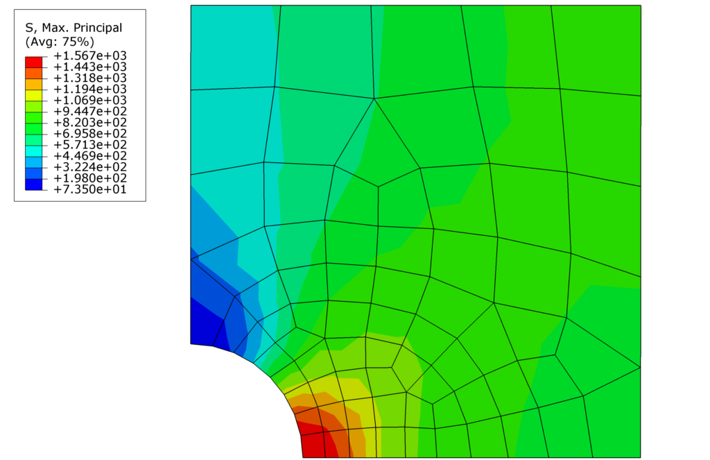
III) Printing field output images
One of the first things you probably do after an Abaqus job is finished is opening the odb file and looking at the von Mises stress field. There are many options for displaying the field output: Different kinds of field output, zoom or rotate the view, cut your model, change the legend and so on. Once you have your view ready, you can print an image from Abaqus (using File/Print), where png images work best (they even have a transparent background). Let’s look at how to automate that, assuming you already know at what angle you want to view what result.
When we want to print nice-looking images, we face two problems in Abaqus: First, depending on the Abaqus window, the aspect ratio of the image will change and second, the legend is usually too small and there is lots of text in the window that we do not want to have in our image:
a) Saving the view
So what can we do concerning the changing aspect ratios of the view window? We give the view window a fixed width and height that we will work with. Run those commands and run them in Abaqus:
vp = session.viewports['Viewport: 1']

# Change size of viewport (e.g. 300x200 pixel)
vp.restore()
# position of the viewport
vp.setValues(origin=(50,-100))
vp.setValues(width=300, height=200)Code language: PHP (php)
Now you have a window with a fixed size and thus aspect ratio. Start recording a macro or use the rpy file in the following: Load your odb and display the results in the way you want. Zoom, drag and rotate your model in the viewport. Once you are happy with what you see, go to View/Save and save your view e.g. as ‘User-1’ with the option Save current.
Now look into your macro or rpy file and copy the commands for loading your odb, showing the results, and saving your view. Since all information about your view is now in the ‘User-1’ view, you can delete all zooming, rotating and dragging commands. Also, add a line for loading the saved view by vp.view.setValues(). After cleaning the code up and adding this line, it should look something like that:
# load the odb
odb = session.openOdb(odb_name+'.odb')

# display the results
vp.setValues(displayedObject=odb)
# show field output, e.g. max. principal stress (INVARIANT/COMPONENT)
vp.odbDisplay.display.setValues(plotState=(CONTOURS_ON_DEF, ))
vp.odbDisplay.setPrimaryVariable(variableLabel='S',
     outputPosition=INTEGRATION_POINT,
     refinement=(INVARIANT, 'Max. Principal'),)

# save view 'User-1'
session.View(name='User-1', nearPlane=150,farPlane=240,width=63,
    height=40,projection=PERSPECTIVE,cameraPosition=(15,0,20),
    cameraUpVector=(0,1,0),cameraTarget=(15,0,0),viewOffsetX=-3.5,
    viewOffsetY=0.02, autoFit=OFF)

# load the defined view
vp.view.setValues(session.views['User-1'])Code language: PHP (php)
If the size of your model geometry can change a lot, using a fixed view is not such a good idea: Then, you can use the default view, save your view with the option Auto-fit (Abaqus automatically zooms so that the hole geometry is in the window) or just use one of the main views like that (access them with View/Toolbars/Views):
vp.view.setValues(session.views['Front'])Code language: CSS (css)b) Formatting the legend and hiding text boxes
In Abaqus, you can go to Viewport/Viewport Annotation Options to change the legend formatting and also select what kinds of text boxes and coordinate systems should be viewed in the viewport. Just do that in Abaqus and record it. My favourite formatting looks like that (hide everything except the legend, white legend background and bigger font size):
# change the legend and what is displayed
vp.viewportAnnotationOptions.setValues(legendFont=
       '-*-verdana-medium-r-normal-*-*-140-*-*-p-*-*-*')
vp.viewportAnnotationOptions.setValues(triad=OFF, state=OFF,
    legendBackgroundStyle=MATCH,annotations=OFF,compass=OFF,
    title=OFF)Code language: PHP (php)
You might need to adapt the view of your model because the legend became bigger. Just do it and copy the new command for saving the view to your script. Finally, we create a png image of the viewport. You can go to File/Print, set everything as you like, record the commands, and copy them to your script. After cleaning them up they might look something like that:
# output image
session.printOptions.setValues(reduceColors=False, vpDecorations=OFF)
# set a bigger image size: 3000 x 2000 pixels
session.pngOptions.setValues(imageSize=(3000, 2000))
session.printToFile(fileName=odb_name+'_max_princ', format=PNG,
		    canvasObjects=(vp,))Code language: PHP (php)
This way, you automatically export an image like that. And you can do so also for hundreds of different load cases in the model. Even with this model, you could think about how to export an image for each frame to see how the stresses become more and more uniform with plastic deformation.
A common error for saving images is that you set the size of the viewport bigger than the screen resolution. So rather take a smaller size of the window but then use
imageSizein thepngOptionsto increase the image size.
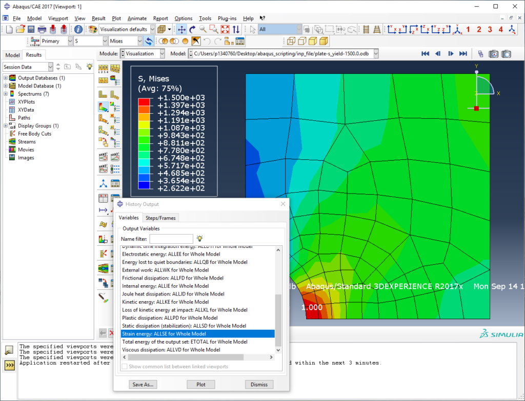
IV) Getting history output data
History output is part of the step object. Between the step and the history output, there is something called historyRegion, which defines what the history output is for (the whole assembly, a contact definition, single nodes, etc.). Let’s look at how to access history output and deal with those regions in more detail.
Once you know the history region where your desired historyOutput is in, you can get the time/result list as I do it here for the whole strain energy of the model ALLSE, which is in the history region with the name ‘Assembly ASSEMBLY’:
step1 = odb.steps['load']

# get time/ALLSE (total strain energy of the model) list
ae_data = np.array(step1.historyRegions['Assembly ASSEMBLY'].
	 	   historyOutputs['ALLSE'].data)Code language: PHP (php)
You can then save your NumPy array containing the history output as we saw it for the field output.
To evaluate multiple steps, you have to obtain the history output for each step separately and then merge them.
But how do we get history output that is not just the default energy of the whole model but for example the displacement of a single node? Writing your step and then .historyRegions[ , and pressing TAB, you can browse through your historyRegions. In one of my models, I found a node that I used for history output:
>>> step1.historyRegions['Node PLATE-1.7814']Code language: CSS (css)Maybe you ask yourself: “How do I know what number my history output node has?”. You don’t, at least not directly! However, you can access the node sets of your instances and find out the node label n_hr in this way:
>>> inst = odb.rootAssembly.instances['PLATE-1']
>>> n_hr = inst.nodeSets['RP'].nodes[0].labelCode language: JavaScript (javascript)
You can then create a string str_hr_node for the historyRegion:
# put together a string to select history region
str_hr_node = 'Node '+inst.name+'.'+str(n_hr)

# get the history region for the node
hr = step1.historyRegions[str_hr_node]Code language: PHP (php)
If you know that there is only one node in the history regions, you can also select this history region by its name like that (using the so-called list comprehension of Python):
hr_node = [hr for hr in step.historyRegions if 'Node' in hr.name][0]Code language: JavaScript (javascript)V) Evaluating results along a path
Sometimes, we want to evaluate field output along a path. Abaqus lets us create paths in the Viewer with Tools/Path/… and can evaluate results along those paths. The basic option is using a list of nodes to define the path.
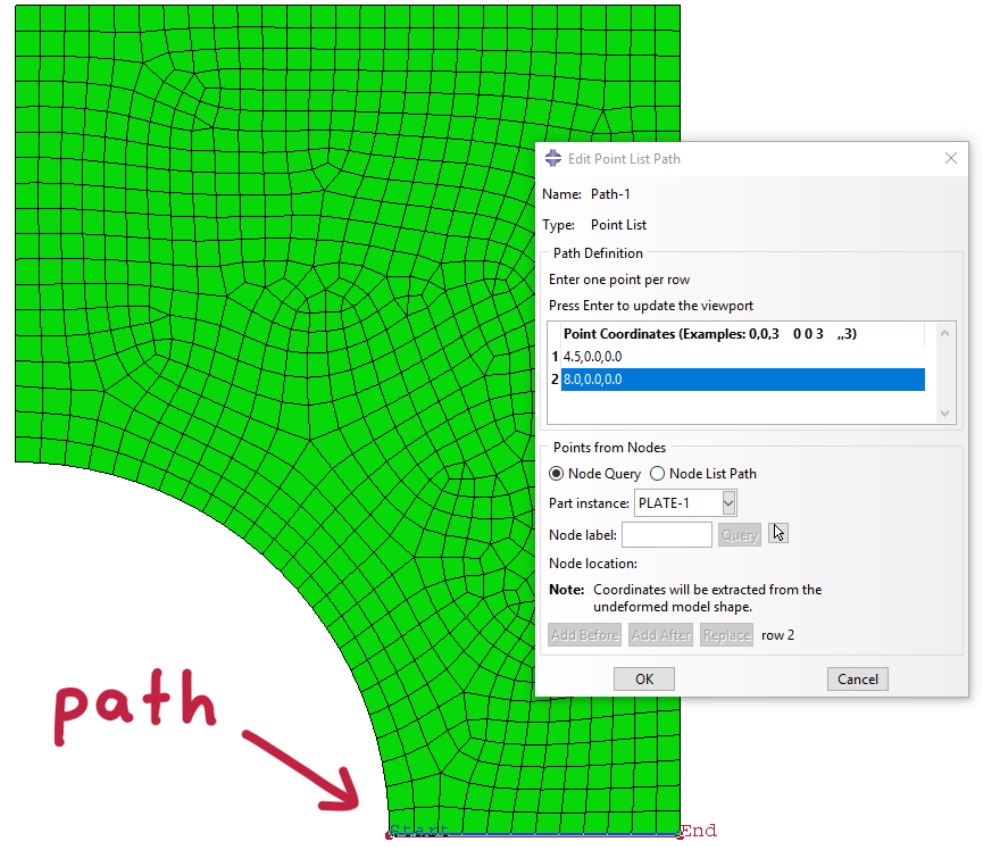
However, it is also possible to define coordinate-based paths. This, for example, creates a path with three points from the point coordinates:
# create path from coordinates
pth = session.Path(name='Path-1', type=POINT_LIST,
                   expression=((0,0,0), (20,0,0), (50,0,0)))Code language: PHP (php)
For the path evaluation, you first have to display the desired field output variable before extracting path results. The first column of the path output can be set by the statement labelType: It can be the distance along the path (TRUE_DISTANCE), the distance projected onto an axis (X_DISTANCE for x-axis) or a coordinate (e.g. X_COORDINATE):
# field output to be evaluated along path
vp.odbDisplay.setPrimaryVariable(variableLabel='S',
    outputPosition=INTEGRATION_POINT,refinement=(COMPONENT, 'S22'))

# output for 20 equidistant points over path
# shape: path over DEFORMED or UNDEFORMED geometry

xy = session.XYDataFromPath(name='XYData-1', path=pth,
    includeIntersections=False, shape=DEFORMED,
    projectOntoMesh=False, pathStyle=UNIFORM_SPACING,
    numIntervals=20, projectionTolerance=0,
    labelType=TRUE_DISTANCE)Code language: PHP (php)
Then you can save your path results xy in a a text file.
Abaqus needs to interpolate result fields if you evaluate paths: You get a value for any coordinate or nothing if the coordinate lies outside your elements. However, this interpolation is rather slow.
Exercises
- Load and run this input file in Abaqus to get the odb file for evaluation. You can do this either in the windows command line by typing
abaqus job=inp_file_nameor by creating a job in Abaqus CAE, selecting source=Input File and then load your inp file. - Evaluate the field output of the displacement
Uand the coordinatesCOORDfor all model nodes and write them to separate dat files. You will need to use the abovegetSubsetfor the coordinates. - Write a script that automatically creates a nice-looking png image of the vertical stress.
- Evaluate the history output of the vertical reaction force RF2 and vertical displacement U2 of the reference point and write those two columns into a dat file.
- Create a path that goes from the notch tip to the right and evaluate the vertical stress S22 over the x-coordinate: a) for undeformed geometry and b) for deformed geometry.
- Load and plot all the dat files in the program of your choice (Origin, Excel, MatLab, Python, etc.). How do the results correspond to the expectations and analytical calculations in chapter 2?